Worked example 2: Your first output
In this section we’ll use biota to generate maps of gamma0 backscatter, AGB, and forest cover. This example covers the 3 forms of biota.
Open Python and import biota
Open a terminal window (right-click the Desktop, and select ‘Open Terminal’), and run the command python or ipython. We recommend use of ipython if available, which has a range of features that make it more user-friendly than standard Python. If successful, you should see something that looks like the following:
To load the biota module, type:
>> import biota
Loading an ALOS tile
Data from the ALOS mosaic is provided as a series of 1 x 1 degree tiles. To load a tile in memory, we need to tell biota what directory the ALOS mosaic data are stored in, and what latitude and longitude we want to load. To save us from writing them out repeatedly, we can store these as variables:
>>> data_dir = '~/DATA/'
>>> latitude = -9
>>> longitude = 38
The biota function to load an ALOS tile can be called with the function biota.loadTile(), which takes inputs of (i) the data directory, (ii) the latitude, (iii) the longitude, and (iv) the year (in this order). Here we’ll load in data for 2007 using the three variables we previously defined:
>>> tile_2007 = biota.LoadTile(data_dir, latitude, longitude, 2007)
The new object called tile_2007 has a range of attributes. These can be accessed as follows:
>>> tile_2007.year
2007
>>> tile_2007.lat
-9
>>> tile_2007.lon
38
>>> tile_2007.directory
'~/DATA/S05E035_07_MOS/'
>>> tile_2007.satellite
'ALOS-1'
>>> tile_2007.xSize, tile_2007.ySize # Raster size, in pixels
(4500, 4500)
>>> tile_2007.xRes, tile_2007.yRes # Pixel resolution in meters
(24.401, 24.579)
Advanced: The tile also contains projection information for interaction with GDAL:
>>> tile_2007.extent # Extent in the format minlon, minlat, maxlon, maxlat
(38.0, -10.0, 39.0, -9.0)
>>> tile_2007.geo_t # A geo_transform object
(38.0, 0.00022222222222222223, 0.0, -9.0, 0.0, -0.00022222222222222223)
>>> tile_2007.proj # Projection wkt
'GEOGCS["WGS 84",DATUM["WGS_1984",SPHEROID["WGS 84",6378137,298.257223563,AUTHORITY["EPSG","7030"]],AUTHORITY["EPSG","6326"]],PRIMEM["Greenwich",0,AUTHORITY["EPSG","8901"]],UNIT["degree",0.0174532925199433,AUTHORITY["EPSG","9122"]],AUTHORITY["EPSG","4326"]]'
There are a few other options that can be specified when loading an ALOS tile, but we’ll return to these in the see the furtheroptions section.
Extracting backscatter information
The biota module is programmed to calibrate ALOS mosaic data to interpretable units of backscatter. This is performed with the getGamma0() function. The data are returned as a masked numpy array:
>>> gamma0_2007 = tile_2007.getGamma0()
>>> gamma0_2007
masked_array(data =
[[0.0669537278370757 0.04214984634805357 0.05141784577914017 ...,
0.029133617952838833 0.024789602664736045 0.040281545637899534]
[0.031600461516752214 0.04214984634805357 0.05141784577914017 ...,
0.03435099209051573 0.028222499657083098 0.03354230142969638]
[0.031600461516752214 0.04050920492690238 0.06216969020533775 ...,
0.037654602824076254 0.04403078198836734 0.025848435873858728]
...,
[0.0900164548052426 0.0662958895217059 0.07768386584418481 ...,
0.049509525268380976 0.0346139149132766 0.021227103665645366]
[0.08548700525257016 0.0888309264753313 0.11198792676214335 ...,
0.08441404357533155 0.06655132961906884 0.05196509713141002]
[0.07134665398730806 0.05708835833035639 0.07595717558689226 ...,
0.021496125937039534 0.027866832136739485 0.0629132766445086]],
            mask =
[[False False False ..., False False False]
[False False False ..., False False False]
[False False False ..., False False False]
...,
[False False False ..., False False False]
[False False False ..., False False False]
[False False False ..., False False False]],
    fill_value = 1e+20)
By default the image loaded is ‘HV’ polarised in ‘natural’ units. It’s also possible to specify options for the polarisation (‘HV’ [default] or ‘HH’) and the units (‘natural’ [default] or ‘decibels’) as follows:
>>> gamma0_HH_2007 = tile_2007.getGamma0(polarisation = 'HH', units = 'decibels')
>>> gamma0_HV_2007 = tile_2007.getGamma0(polarisation = 'HV', units = 'decibels')
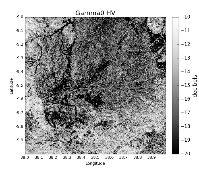
If we want to visualise this data, we can run:
>>> gamma0_2007 = tile_2007.getGamma0(polarisation = 'HV', units = 'decibels', show = True)
Which produces the following image:
If we want to save this data to a geoTiff, we can run:
>>> gamma0_2007 = tile_2007.getGamma0(polarisation = 'HV', units = 'decibels', output = True)
This will write a GeoTiff file to the current working directory. This file can be processed and visualised in standard GIS and remote sensing software (e.g. QGIS, GDAL).
To load these tiles and save a raster of backscatter through the command line, run:
biota snapshot -dir /path/to/data/ -lat -9 -lon 38, -y 2007 -o Gamma0 -lf
To change the default polarisation setting, add the flag -pz and enter the desired polarisation. For instance, to get ‘HH’ data:
biota snapshot -dir /path/to/data/ -lat -9 -lon 38, -y 2007 -o Gamma0 -lf -pz HH
NB; biota does not support data visualisation in the command line, as many users will not have a graphic interface from their terminal. To visualise DATA, load the output raster in GIS software or plot it with Python.
Building a map of AGB
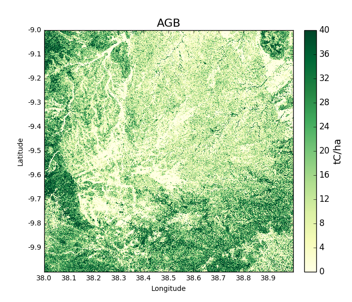
In a similar way to loading gamma0 backscatter, we can show maps of AGB.
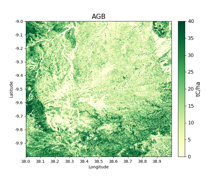
>>> agb_2007 = tile_2007.getAGB(show = True)
Areas in darker green show denser forest:
Like the previous function (and most others in the biota module), we can output a GeoTiff as follows:
>>> agb_2007 = tile_2007.getAGB(output = True) # To output AGB map to a GeoTiff
Or, from the command line, run:
biota snapshot -dir /path/to/data/ -lat -9 -lon 38, -y 2007 -o AGB -lf
Note
By default biota uses an equation calibrated for ALOS-1 in miombo woodlands of Southern Africa. It’s advisable to have a locally calibrated biomass-backscatter equation to improve predictions.
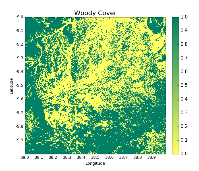
Building a forest cover map
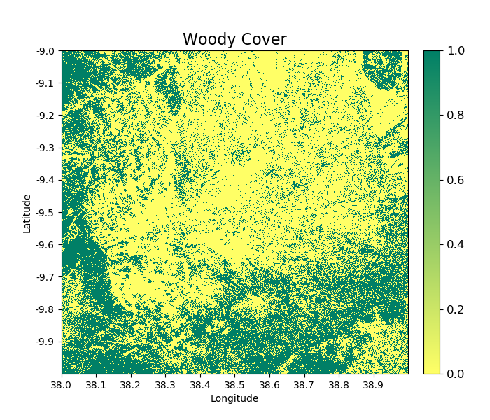
A forest cover map (or ‘woody cover’) can be generated as follows:
>>> woodycover_2007 = tile_2007.getWoodyCover(show = True)
and output:
>>> woodycover_2007 = tile_2007.getWoodyCover(output = True)
To execute this from the command line, run:
biota snapshot -dir /path/to/data/ -lat -9 -lon 38, -y 2007 -o WoodyCover -lf
By default biota will use a generic definition of forest of 10 tC/ha with no minimum area. In the next section we’ll discuss how this and other forest definitons can be customised.
Further options when loading an ALOS tile
biota supports a range of options for data processing and forest definitions. These options should be specified when loading a tile. These various options can be specified in any combination, but be aware that when analysing change the pre-processing steps for each tile should be identical.
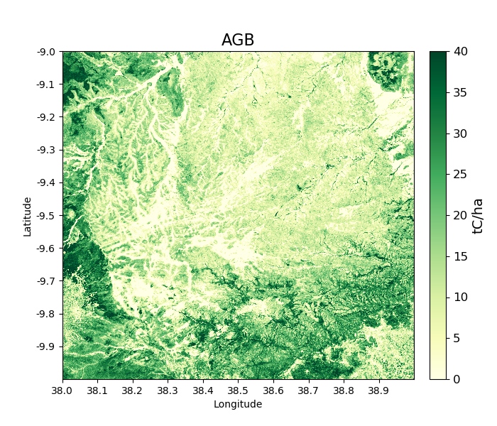
Speckle filtering
Radar data are often very noisy as the result of ‘radar speckle’, which can be supressed with a speckle filter. The biota module has an Enhanced Lee speckle filter, which can be applied to the ALOS tile. By default, no filtering is applied. The speckle filter should be specified on loading the tile:
>>> tile_2007 = biota.LoadTile(data_dir, latitude, longitude, 2007, lee_filter = True)
Filtering results in an AGB map is noticeably less noisy than those from unfiltered ALOS image.
>>> tile_2007.getAGB(show = True)
In the command line, the flag -lf deactivates the speckle-filtering (ON by default). To keep the filter on, simply do not type the flag:
biota snapshot -dir /path/to/data/ -lat -9 -lon 38, -y 2007 -o AGB
Downsampling
Data volumes can be reduced through downsampling. This comes at a cost to resolution, but does have the positive effect of reducing speckle noise. By default, no downsampling is appied. For example, to halve the resolution of output images, set the parameter downsample_factor to 2:
>>> tile_2007 = biota.LoadTile(data_dir, latitude, longitude, 2007, downsample_factor = 2)
With a downsample_factor of 2, the resolution of the image is halved:
>>> tile_2007.getAGB(show = True)
In the command line, the flag -ds activates downsampling and is followed by the downsampling factor. To reproduce the result above, run:
biota snapshot -dir /path/to/data/ -lat -9 -lon 38, -y 2007 -o AGB -lf
Changing forest definitions
For many purposes it’s useful to classify regions into forest and nonforest areas. To achieve this with biota a threshold AGB (forest_threshold) and a minimum area (area_threshold) that separate forest from nonforest can be specified. By default the forest_threshold is 10 tC/ha and the area_threshold is 0 ha. For example, for a forest definition of 15 tC/ha with a minimum area of 1 hecatare:
>>> tile_2007 = biota.LoadTile(data_dir, latitude, longitude, 2007, forest_threshold = 15, area_threshold = 1)
A higher forest_threshold or minimum_area results in a reduced forest area:
>>> tile_2007.getWoodyCover(show = True)
In the command line, the flag - activates downsampling and is followed by the downsampling factor. To reproduce the result above, run:
biota snapshot -dir /path/to/data/ -lat -9 -lon 38, -y 2007 -o WoodyCover -lf -ft 15 -at 1
Changing output directory
By default, GeoTiffs are output to the current working directory. This may not be the best place to output GeoTiff files, a different output directory can be specified as follows:
>>> tile_2007 = biota.LoadTile(data_dir, latitude, longitude, 2007, output_dir = '~/output_data/)
From the command line: .. code-block:: console
biota snapshot -dir /path/to/data/ -lat -9 -lon 38, -y 2007 -o WoodyCover -lf -od /path/to/output/
Masking data
The ALOS mosaic product is supplied with a basic mask indicating locations of radar show and large water bodies. For many applications this may not be sufficient. For example, radar backscatter from ALOS is strongly influenced by soil moisture changes, which will be particularly severe around rivers.
For some biomass mapping applications and for change detection, we might want to mask out rivers or other features. The biota library can generate an updated mask with either classified GeoTiffs or shapefiles.
NB: biota does not support masking from the command line, since it does not output direct visualisations.
Masking with a shapefile
For this example, we’ll use a publically available shapefile of inland water in Tanzania from Diva GIS. Download the shapefile here, unzip it, and save it somewhere accessible.
This can be done on the command line as follows:
mkdir auxillary_data
cd auxillary_data
wget http://biogeo.ucdavis.edu/data/diva/wat/TZA_wat.zip
unzip TZA_wat.zip
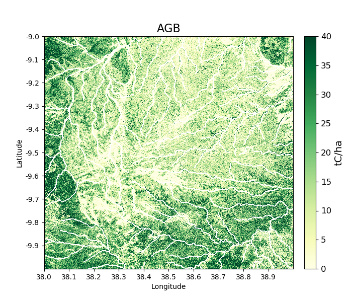
We can use this shapefile to update the mask in biota, applying a 250 m mask around river lines, as follows:
>>> tile_2007.updateMask('auxillary_data/TZA_water_lines_dcw.shp', buffer_size = 250)
River lines and 250 m buffer now appear in white in the resultant image:
>>> tile_2007.getAGB(show = True)
Masking with a GeoTiff
Perhaps we aren’t interested in mapping known agricultural land, we might want to mask out areas of agriculture from a land cover map.
Here we’ll use the ESA CCI land cover map to locate areas of agriculture. The 2007 map is available to download from ESA.
With the command line:
cd auxillary_data
wget ftp://geo10.elie.ucl.ac.be/v207/ESACCI-LC-L4-LCCS-Map-300m-P1Y-2007-v2.0.7.tif
In the ESA CCI data product the values 10, 20, 30, and 40 correspond to locations with agriculture. We can mask out this class in biota as follows:
>>> tile_2007.updateMask('auxillary_data/ESACCI-LC-L4-LCCS-Map-300m-P1Y-2007-v2.0.7.tif', classes = [10, 20, 30])
Areas to the south-west of the image now appear in the white mask.
>>> tile_2007.getAGB(show = True)
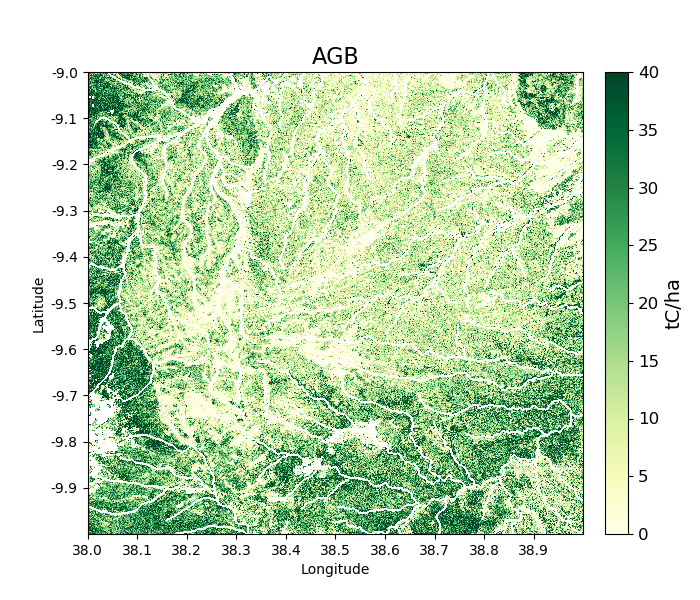
Note, that the updateMask() function added to the previous water mask rather than replacing it. updateMask() can be run multiple times to make use of multiple datasets.
Putting it all together
Using the commands above, we can create a script to automate the pre-processing of an ALOS tile to generate outputs of gamma0 (HV backscatter in units of decibels), AGB and forest cover for the year 2007. We’ll filter the data and specify a forest threshold of 15 tC/ha with a minimum area of 1 hectare, Using a text editor:
# Import the biota module
import biota

# Define a variable with the location of ALOS tiles
data_dir = '~/DATA/'

# Define and output location
output_dir = '~/outputs/'

# Define latitude and longitude
latitude = -9
longitude = 38

# Load the ALOS tile with specified options
tile_2007 = biota.LoadTile(data_dir, latitude, longitude, 2007, lee_filter = True, forest_threshold = 15., area_threshold = 1, output_dir = output_dir)

# Add river lines to the mask with a 250 m buffer
tile_2007.updateMask('auxillary_data/TZA_water_lines_dcw.shp', buffer_size = 250)

# Calculate gamma0 and output to GeoTiff
gamma0_2007 = tile_2007.getGamma0(output = True)

# Calculate AGB and output to GeoTiff
gamma0_2007 = tile_2007.getAGB(output = True)

# Calculate Woody cover and output to GeoTiff
gamma0_2007 = tile_2007.getWoodyCover(output = True)
Save this file (e.g. process_2007.py), and run on the command line:
Advanced: To process multiple tiles, we can use nested for loops. We can also add a try/except condition to prevent the program from crashing if an ALOS tile can’t be loaded (e.g. over the ocean).
# Import the biota module
import biota

# Define a variable with the location of ALOS tiles
data_dir = '~/DATA/'

# Define and output location
output_dir = '~/outputs/'

for latitude in range(-9,-7):
    for longitude in range(38, 40):

        # Print progress
        print 'Doing latitude: %s, longitude: %s'%(str(latitude), str(longitude))

        # Load the ALOS tile with specified options
        try:
            tile_2007 = biota.LoadTile(data_dir, latitude, longitude, 2007, lee_filter = True, forest_threshold = 15., area_threshold = 1, output_dir = output_dir)

        except:
            continue

        # Add river lines to the mask with a 250 m buffer
        tile_2007.updateMask('auxillary_data/TZA_water_lines_dcw.shp', buffer_size = 250)

        # Calculate gamma0 and output to GeoTiff
        gamma0_2007 = tile_2007.getGamma0(output = True)

        # Calculate AGB and output to GeoTiff
        gamma0_2007 = tile_2007.getAGB(output = True)

        # Calculate Woody cover and output to GeoTiff
        gamma0_2007 = tile_2007.getWoodyCover(output = True)
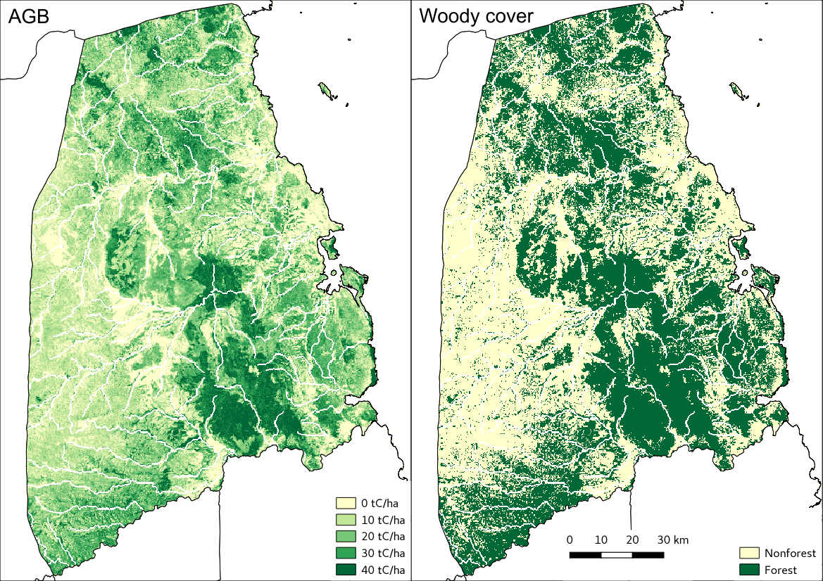
Visualised in QGIS, the resulting biomass and woody cover maps for Kilwa District are:
Producing an output with the GUI
once the window is open, select a Latitude and Longitude, then ‘Forest property’. Select the year for which you want to donwload and process the data (yes, the download is automatic in the GUI) and tick the boxes you want to output. If you want to refine your analysis, modify the Area threshold and the Biomass threshold. That’s it!